Your everyday world from a physicist's perspective
A story of a rubber band
Take a rubber band (a rubber balloon also works), hold it against your forehead or lips, and stretch it all the way. Hold it for a while and then let it relax again.

Besides the strange looks from the people in your direct environment, you will notice two things:
- The more you stretch the rubber band, the harder it pulls back;
- When the rubber bands is completely stretched it feels slightly hotter than before, and upon release, it immediately cools down again.
The second effect is not very big, but because your forehead and lips are pretty decent thermometers you can feel the difference (it works better if you wet your lips a bit).
Although this phenomenon might not seem as spectacular as the specular colors and water bells in the previous articles, I ask you to be patient and give the humble rubber band a chance to reveal its deepest grounds, its relation to life and to the rest of the universe (!)
What is the chance of that!?
At times, things appear to be quite easy going from our big mammal perspective, but when we zoom in far enough at any piece of the world, we'll find that things are always rushing around at the microscopic level. Just for the fun of it, try to imagine the octillions and octillions of air molecules bombarding us every second from all possible directions (about 5000000000000000000000000000 impacts per second for an average human body to be precise).
With this picture in mind, let us try to cook up a representative microscopic model of a rubber band.
A toy model of a rubber band
Industrial rubber consists of a "spaghetti network" of long polymer chains that is given some robustness by a process called 'vulcanization'. In this process sulfide bonds are formed between the polymers, connecting the spaghetti chains together at some places. Where there are no such bonds, the chains can still kink and curl up as much as they want.
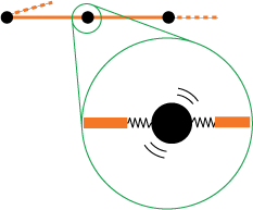
In our rubber band model we will simplify this picture by saying that the rubber band is made of stiff "molecules" of equal length l, chained together by rotatable hinges, so that each molecule can point either to the left or to the right (see figure 1).
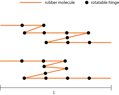
Now, let's try to find out how such a "kinky system" will behave to the eye of the (macroscopic) beholder.
Dynamic equilibrium
First have a look at figure 2. In this picture a small metallic ring is suspended between two partially stretched rubber bands. As one can tell from the photo, the metallic ring finds a stable position somewhere halfway between the two bands. If we move the ring a bit to the left or to the right and then release it, it will immediately return to its former position.
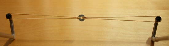
From a macroscopic point of view this behavior is easy to understand: the ring finds a equilibrium position where the rubber band on the left pulls with the same force as the band on the right. But how can we understand this behavior from our microscopic picture?
Remember: it is always rush hour in the world of atoms and molecules. So if we start out with a nicely straightened chain of rubber band molecules, it surely won't stay straight for long. The bombardment by air molecules will introduce kinks in no time. To get a more quantitative idea of this kinking behavior, let us make a bold assumption about its statistics.
- We will say that every microscopic realization of the chain that meets the imposed constraints (say a certain total length), is equally likely to occur.
This single assumption (!) is the backbone of one of the biggest areas in physics, called (you could have guessed it) 'statistical physics'. Actually, one has to add some conditions like that there is no energy (or anything else) transfered back or forward between the rubber band and its environment (we have to put it in a sealed box, etc), but I won't bother you with this now, as it is not important for the general idea.
Finding the most probable macro state
Let us return to our little metallic ring that is still floating seemingly comfortable between the two rubber bands. First we note that the total length L of the two rubber bands is fixed. If we denote the length of the first rubber band by L1 and that of the second band by L2, this can be stated mathematically as
(1) .
.
Because L1 and L2 determine the position of the ring (the thing we big mammals are interested in) we will call each combination of (L1, L2) a possible 'macro state'. In what follows I will (for convenience) always express lengths in terms of the rubber molecule length l. So if I say L1 = 5, I mean that the length of the first rubber band is five times that of a single rubber molecule.
To complete the set of constraints for our rubber bands we also have to specify the total number of molecules (N1, N2) they contain. It is clear (from figure 1) that we must always have N > L.
Now, in order to put our bold statistical assumption to good use, we set out to find for each possible combination of L1 and L2, the number of microscopic ways in which it can happen. Because if we know the number of microscopic realizations for each macro state, we can (upon mutual comparison) find the most probable one.
Let us work out a small example for a single rubber band of length L1 = 3 and containing N1 = 7 molecules. If we denote a forward pointing rubber band molecule by an 'f' and a backward pointing molecule by a 'b' we can easily figure out all the possible ways in which we can arrange the seven molecules in order to get a length of 3:
- fffffbb, ffffbfb, ffffbbf, fffbffb, fffbfbf, fffbbff, ffbfffb, ffbffbf, ffbfbff, ffbbfff, fbffffb, fbfffbf, fbffbff, fbfbfff, fbbffff, bfffffb, bffffbf, bfffbff, bffbfff, bfbffff and bbfffff.
We count 21 possible microscopic realizations of the macro state L1 = 3 (N1 = 7). Note that each string contains exactly (N1 + L1) / 2 = 5 forward pointing molecules and (N1 - L1) / 2 = 2 backward pointing molecules. This fact allows us to take a mathematical shortcut to find the number of realizations. If you open any book on statistics, it will tell you that the number of distinct ways in which you can stack five "forestgreen coins" and two "blue coins" is equal to
(2) ,
,
where 7! means, do 7*6*5*4*3*2*1 (mathematicians call this 'the factorial of 7'; similarly 5! = 5*4*3*2*1, you get the idea...).
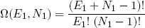
For arbitrary N1 and L1 we have
(3)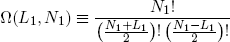 .
.
Ω is called the 'multiplicity' of the band. The same expression holds for the second band (with the subscript '1' replaced by '2' of course).
To find the number of microscopic realizations for the two bands tied together, we can simply multiply the multiplicities of the separate bands (see that same textbook on statistics),
(4) .
.
With our constraint L = L1 + L2 we can also write this as
(5) ,
,
where L1 can vary between 0 [metallic ring all the way to the left] and L [ring all the way to the right].
Figure 3 shows a graph of Ωtot versus L1 (with N1 = 600, N2 = 400 and total length L = 500).
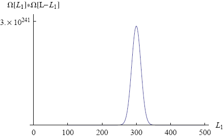
We immediately see that there is one value of L1 (namely L1 = 300) around which the total number of microscopic realizations is tremendously big (of the order of 10241). This means that if move the ring to a position of lower multiplicity (L1 = 200, say) and then release it, the chance is overwhelming that we will find it close to L1 = 300 if we look some time later.
Note that the rubber band in our example consists of "only" a thousand molecules. In a real rubber band the number of molecules is closer to 1023. For such a rubber band the peak in the multiplicity graph will be unimaginably high. On a human scale it will look like a thin line at a single value of L1, the equilibrium position of the ring. In principle there is a chance that the ring spontaneously moves all the way to one side, but it just won't happen within the lifetime of the universe (or any multiple of that).
To sum up: to find the equilibrium position of the metallic ring between the two rubber bands, we first figured out the number of microscopic realizations (the 'multiplicity') for each position. It turned out that this multiplicity has a well defined peak at one specific ring position. Since we assumed that each microscopic state is equally probable, we could then argue that this is the position that will be observed (with overwhelming probability). Basically this is all there is to statistical physics. Let's see what we can get out of it.
Energy juggling - the same argument all over again
Up till now the rubber band molecules are still a bit too passive to my taste. To make things more realistic and to be able to understand the heat effects of the rubber band later on, we extend our simple model to take into account the vibrations of the molecules. We picture that each molecule is attached to its hinge base by a little spring (see figure 4).
Of course there are no such springs in reality (as far as I know), but the electrostatic forces result in very similar behavior (and besides that, the actual mechanism does not really matter in the argument that follows). The important point is that each molecule can store a certain amount of vibrational energy. And in fact it is this inherent vibrational motion that mainly drives the random kinking of the rubber band (so the rubber band also works in a vacuum!).
To make it easier to "count the energy", we assume that each molecule can only store energy in lumps of a definite amount q (actually, quantum mechanics tells us that this is the way it really is!). So we would say something like: "the sixth molecule from the left vibrates with 3 lumps of vibrational energy."
We can schematically depict a certain distribution of vibrational energy over the molecules as follows,
**|***|****||* ,
where the dots '*' represent lumps of energy and the vertical bars '|' represent separation lines between the molecules. So here we have 2 lumps of energy on the first molecule, 3 on the second, 4 on the third, none on the fourth and one on the last.
From this picture we can immediately write down the multiplicity of distributing E1 lumps of energy over N1 molecules (analogous to equation 3):
(6)
and for our two connected rubber bands we have
(7) ,
,
where we used that the total energy E1 + E2 = E is held fixed. If we make a graph of this equation (with N1 = 300, N2 = 200, E = 500; see figure 5) we find a shape that looks very familiar.
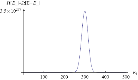
Again a peak shows up around one specific value of the macroscopic parameter. We see that the most likely energy distribution is 300 energy packets on the first band and 200 packets on the second band. In this situation both bands have the same average energy per molecule (as one might have expected). We say that the two bands are in 'thermal equilibrium' for this value of E1.
If I say 'thermal equilibrium' you probably think 'equal temperature'. And you are quite right. But what exactly is temperature? What do we mean if we say "Drink your coffee while it is still hot."? Physicists have come a long way since that question was first posed, but before I can tell you their answer, we will first need a bit more mathematical trickery (don't worry, this should look familiar from high school).
Intermezzo: Handling huge numbers
Even for a modest amount of molecules, the number of possible arrangements (i.e. the multiplicity) tends to be HUGE. Luckily for us the mathematics department came up with a nifty way to keep big numbers manageable. They call it 'the logarithmic scale'. Basically the logaritm of some number 'a' (written as log(a)) is defined as the value 'b' for which
(8) ,
,
where e is a fancy constant called Euler's number (approximately equal to 2.71828; one can also use a different base, but this is the convention).
Example: on the logarithm scale, the huge multiplicity found in the previous section for the number of energy packet distributions reduces to
(9)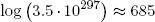 .
.
Another big advantage of the logarithmic scale (and essentially the reason why huge numbers become manageable on this scale), is that it effectively converts multiplication to addition. In mathematical notation we say
(10) .
.
Thus if we look at the logarithm of the combined multiplicity of our two rubber bands, we can now simply add the logarithms of multiplicity of the separate bands (instead of multiplying the multiplicities - can you still follow?)
(11) .
.
Last but not least there is a very neat trick - called 'Stirling's approximation' - to calculate the logarithm of the factorial of a big number, it reads
(12)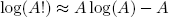 ,
,
and works best for A > 100.
Entropy
If you are getting tired and bored of reading 'the logarithm of multiplicity' all the time, don't worry, from now on I will simply call it 'the entropy' (this is what physicists call it since 1865). In mathematical formulas we denote entropy by the symbol S.
Back to our rubber bands. If we take the logarithm of equations 3 and 6 and exploit the tricks from the previous section, we can write down neat expressions for the length and energy entropies of a single rubber band (as a function of N, L and E):
(13)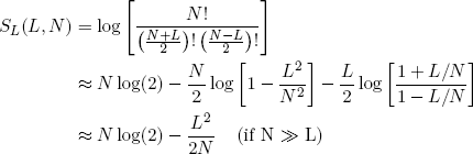
and
(14) .
.
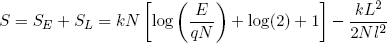
The total entropy of a single rubber band is then given by S = SE + SL (remember: we can add entropies where we would multiply multiplicities) and the total entropy of the two bands tied together is
(15) .
.
You get the idea.
Temperature
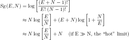
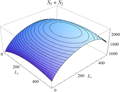
In figure 6 I plotted the total entropy of the rubber bands as function of E1 and L1 (equation 15; keeping the total length and energy fixed as before). Because of the nature of the logarithm function, the maximum of the entropy will coincide with the maximum of the multiplicity from which it was derived (but note that the peak is not as sharp because of the logarithmic scale).
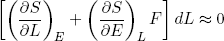
One can find the maximum of a function by finding the point where its slope is zero (along both axes). In mathematical notation we say (for the L1 and E1 direction):
(16)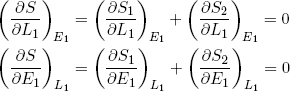 .
.
The curly d's (∂) indicate that the derivative is with respect to only one of the variables, while the subscripts next to the brackets indicate the variables that are held fixed (maybe a bit redundant, but in thermodynamics it is a good practice to keep track of these things carefully).
From the imposed constraint of fixed total energy (E1 + E2 = const) it follows that a decrease in the energy of one band must equal the increase in energy in the other band. This means that we can also write the last expression as
(17) ,
,
where we substituted ∂E1 by -∂E2 and sneakily replaced L1 by L2 in the second term (which is perfectly fine since L1 + L2 = const). Carrying the second term over to the right side of the equality sign we get
(18) (at equilibrium).
This expression says that the slopes (in the E direction) of the entropies of the separate bands are equal when the bands are in thermal equilibrium. Note that the term on the left only contains variables referring to the first rubber band, while the term on the right only has variables belonging to the second band. So we can call this "thing" a genuine property of a single rubber band. This "thing" turns out to be what we usually refer to as the temperature (isn't that exciting?). Nowadays physicists even go a step further and take it as the definition of temperature (actually we take 1 over the thing, to make "hot" correspond to large T).
So instead of equation 18 we write
(19) (at equilibrium),
with
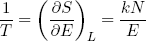
(20)  .
.
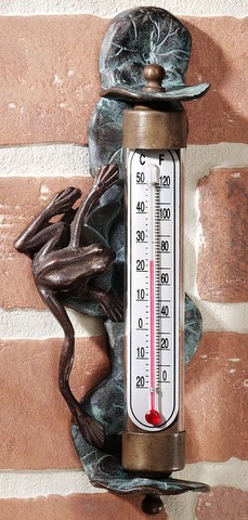
Some substances have the property that their volume increases more or less linearly with temperature. This explains the success of for example the mercury-in-glass thermometer from early times (see figure 7) and the tea experiment.
To get the temperature in the scale and units we measure with a thermometer (plus an offset of 273.15 degrees), we have to multiply the entropy by a historical pre-factor of k = 1.380648×10⁻²³ J/K, in other words S ≡ k log(Ω).
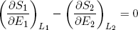
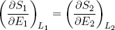
In the discussion above we focused on the derivative of entropy with respect to energy, but similar arguments hold for the slope along the length (L) axis. Because ∂L1 = -∂L2, we have from the first equality in equation 16 that
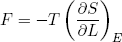
(21)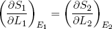 (at equilibrium).
We will see later that this quantity is directly related to the force a rubber band exerts, but first we will look a bit closer at the idea of hot versus cold and the direction of spontaneous heat flow.
Irreversibility - a cup of tea does not get hot by itself
As we argued before in terms of multiplicity: any system that starts out in a macroscopic state not corresponding to the maximum total entropy, tends to move (by cheer chance) uphill to a state of higher and higher entropy. In view of equation 20 for the definition of temperature, this means for example that if we place a hot object (low slope) in contact with a cold object (high slope), the total entropy can (and will) increase by transferring energy from the hot object (moving downhill a bit) to the cold object (moving uphill a bit more). In other words: we can understand the temperature as a measure of how bad an object "wants" to give up energy.
Once something is on top of the entropy hill, the odds are (very) negligible that we will ever see it spontaneously move down again. Such a process is called 'irreversible'. A cup of tea (or a rubber band for that matter) never spontaneously gets hot again after it has cooled down by being in contact with the "cold" air! Just as our suspended metal ring never moves all the way to one side or the other after it has found its equilibrium position.
Physicists and engineers found this observation so profound that they bombastically called it 'the second law of thermodynamics' (the first law being the conservation of energy). In any spontaneous process, the total entropy in the world must increase.
Adiabatic stretching - putting entropy to good use!
Let's put some action into the game. If you stretch a rubber band you'll notice that it really "wants" to go back to its equilibrium position (by pulling back on you). Now we would like to put this "urge to do something" to good use; e.g. move something around, shoot something at the teacher, whatever. In other words, we want to convert the pull to a directed form of energy, called 'work'.
When the band does work (on whatever), it must lose an equal amount of energy (from the general principle of energy conservation). This energy must come from the stored vibrational energy. If the band is isolated from the environment, a loss of vibrational energy also implies a decrease in the entropy of the band (according to equation 14). Still, we want the band to move back spontaneously. So by the second law, the total entropy should increase. This net increase in entropy is provided in by a decrease in the length of the rubber band (equation 13).
It is easy to see that the best we can do (to still have it go) is to have the "energy entropy" decrease by an amount almost equal to the increase in "length entropy". So in the case of a relaxing the rubber band (getting out some work) we have
(22) .
.
Now suppose we want to reverse the motion and stretch the rubber band. This time we have to put in at least enough work to overcome the urge to move back, and a bit more to make it go comfortably. Thus we have a decrease in the length entropy (we are making it longer) and a slightly bigger increase in the vibrational energy entropy (we are putting in energy),
(23) .
.
Conclusion: in both cases the change in entropy is (at least slightly) positive.
In the book by Landau and Lifshitz (two famous physicists from Russia) they give a beautiful argument to show that one can make the increase in entropy as small as one wants (thus being more efficient) by releasing or stretching the rubber band "sufficiently slowly". I'll outline the idea shortly: suppose we are slowly changing some macroscopic parameter λ (the length of the band in our example) so that dλ/dt is small, then we can at any time 'expand' the corresponding rate of change in the total entropy dS/dt in powers of dλ/dt (known from calculus as a 'Taylor expansion')
(24)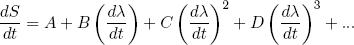 ,
,
where A, B, C, D etc. are some constants not depending on dλ/dt. Since dλ/dt is supposed to be small, each next term in the power series will be an order of magnitude smaller. So to find the dominant term we have to find the first constant that is not zero.
Let's put in some physics: if dλ/dt = 0 we must have dS/dt = 0 (nothing is changing), so we immediately see from equation 24 that A = 0. The second term can be positive or negative (depending on the sign of dλ/dt), but we argued before that the change in entropy must be positive no matter in which direction we let the length change. To make sure we have this behavior, B must be zero too. This means that the dominant term is the one quadratic in dλ/dt,
(25)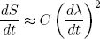 ,
,
or, by rearranging the dt's and dλ's a bit (we are not mathematicians),
(26) .
.
This shows that we can make dS/dλ (the change in S upon changing λ) as small as we want by decreasing dλ/dt. Such sufficiently slow stretching or relaxing of an isolated rubber band is called 'adiabatic stretching or relaxing'.
We can use this concept of adiabatic change to prove a relation between the force a stretched rubber band exerts and the derivatives of the entropy. From calculus we know that if we have an infinitesimal (very small) change in the variables L and/or E of some function S(L, E) then the corresponding change in S is given by
(27)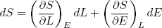
If we change the length adiabatically (i.e. very slowly while keeping it isolated) we must also have
(28)
Furthermore we know (from high school) that the work we have to put in (or get out) is equal to the force F we have to apply (or is applied to us), times the distance dL we move,
(29)
Combining this expression with equations 27 and 28 we find
(30)
or
(31)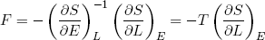
The force we feel (if we move sufficiently slowly, or not at all) is directly related to the temperature of the band and the slope of its entropy in the L direction.
The rubber band law
In the last sections we figured out a relation between force and temperature and derivatives of the entropy. From our microscopic picture we calculated the entropy of a rubber band. Let's put one and one together and see what comes out. We start with the force,
(32)
and (in the hot limit)
(33)
where we tagged on the pre-factor k and converted to units in which we measure L in meters (by replacing L by L/l) and E in joules (by replacing E by E/q). Taking the derivative with respect to L (keeping E constant) gives
(34) .
.
The force varies linear with temperature (at fixed length) and linear with length (at fixed temperature). We could call this equation the 'ideal rubber band law', as it happens to be the exact analog of the famous 'ideal gas law'
(35) ,
,
in which P and V are respectively the pressure and the volume of the gas.
Another useful relation can be found if we calculate the temperature using equation 20 in combination with our expression for the entropy (equation 33),
(36)
or
(37) .
.
This equation says that the total energy stored in the rubber band is equal to the number of molecules N times the quantity kT. In other words, in this case the temperature (times k) can also be interpreted as the average energy per molecule. This turns out to hold quite generally in the hot limit (kT >> q). For lower temperatures (or bigger "energy packets") the quantization begins to play an important role.
Time for the grand finale.
Heat engines, refrigerators, life and the rest of the universe
Besides for shooting paper bullets, rubber bands can also be used to make a genuine 'heat engine' (see the very instructive movie by Adam Micolich below).
In a heat engine random vibrational energy is converted into work (directed energy). Now, it turns out that it is not possible to take random energy (i.e. heat) at a single temperature and convert it into work in a cyclic manner (to make an engine for example).
So what can we do? We know that energy spontaneously "flows" from a hot object to a cold object, so maybe we can "tap" into this flow and get out some useful work. We will need two 'heat reservoirs', one hot and one cold and some kind of 'medium' to convert the flow of heat into work (a rubber band for example). A possible (though idealized) implementation of such an engine is the so called 'Carnot cycle' shown schematically in figure 8.
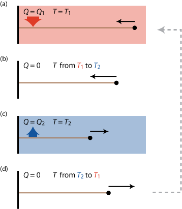
Starting from a stretched rubber band, the Carnot cycle consist of the following steps
- relaxing the band within the hot reservoir; slowly to keep the temperature of the band approximately equal to that of that reservoir along the way (by a spontaneous heat flow Q1 into the rubber band that would otherwise cool down),
- isolating the band from the environment and relaxing the band adiabatically, so that it can cool down to the temperature of the cold reservoir,
- stretching the band again in the cold reservoir; keeping it at the same temperature by a spontaneous heat flow Q2 out of the band,
- isolating the band and adiabatically stretching it back to its original length and temperature.
How much net work W can we get out of this engine in one cycle? In the first step an amount Q1 of heat energy goes in, in step (c) an amount Q2 flows out. If we assume that besides work and heat, no other forms of energy are exchanged and if we believe that energy is conserved, then, since 'energy in' equals 'energy out', we can write
(38) ,
,
or
(39) .
.
So to find the net work that can be produced in a Carnot cycle, we have to figure out how much heat is transfered from and to the heat reservoirs in the 'isothermal' (constant temperature) steps (a) and (c).
Equation 37 tells us that constant temperature also means constant energy. On the other hand, when the rubber band is doing work (or work is being done on it), it tends to lose (or gain) energy. In order to keep the temperature constant, this energy must be replenished (or drained) by transferring an equal amount of heat from (or to) the heat reservoir. In other words
(40)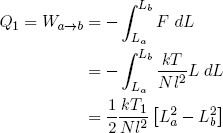 ,
,
where we used the ideal rubber band law on the second line, and similarly
(41)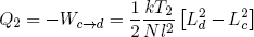 .
.
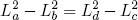
To compare Q1 and Q2 we still need a relation between [La2 - Lb2] and [Ld2 - Lc2]. We can get this relation by calculating how much the length changes in the adiabatic relaxation and stretching steps (b and d) that connect temperatures T1 and T2.
For an adiabatic change in the length of our ideal rubber band we have
(42)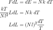 .
.
We can integrate on both sides of the equality sign to find
(43)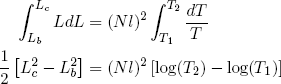
for stretching from (b) to (c), and
(44)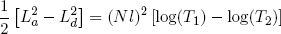
for (d) back to (a). Comparing these expressions gives the relation we set out for
(45) ,
,
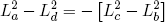
or
(46)
 .
.
Using this relation in equations 40 and 41 for the heat in- and output, we conclude
(47) .
.
In engine design one is often interested in the efficiency of a motor, defined as 'work out' over 'heat in'. For our Carnot cycle we find
(48) .
.
where T1 is the temperature of the hot reservoir and T2 is the temperature of the cold reservoir. One can immediately see that the bigger the difference in temperature, the higher the efficiency. This is a very important rule in engine design.
Can we do better than the Carnot cycle?
Management summary: no
Long answer: the Carnot cycle represents a very special kind of engine: namely a reversible engine. This means that one can run it in reverse: putting in work W, taking out an amount Q2 from the cold reservoir and disposing an amount Q1 into the hot reservoir. In other words, we can use it as a refrigerator! In the ideal (i.e. "frictionless") case we could take two Carnot cycles, one running in reverse on the work produced by the other, and have it in such a way that the energy in the reservoirs remains (more or less) unchanged. The Carnot cycle has this property because we made sure that the rubber band is near (thermal) equilibrium at all times (so that no irreversible processes occur).
Carnot (the famous French military engineer, who lived in the 19th century) published a beautiful argument to show that a heat engine that is perfectly reversible (hypothetically or not), cannot be beaten when it comes to efficiency, no matter how the other engine is build.
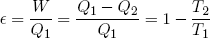
Basically he assumed (based on experience) that it is not possible to take heat at a single temperature and convert it into work (continuously). Then he asks: what if we had an engine that is more efficient than a reversible engine? We could then take a part of the work produced by this "super motor", and use it in a reversible engine to keep the energy in the cold reservoir unchanged (see figure 9). The rest of the work we could use to do something else. We would (effectively) have taken heat at a single temperature and converted it into work, which contradicts our initial assumption. Conclusion: a more efficient heat engine is not possible!
Although the Carnot cycle is very efficient, it is not very practical (because it is very slow) and it is therefore mainly used as a reference for real engines.
What makes our world go?
If there would exists a single heat engine that can keep all the processes on our planet up and running, it must be huge. And it is.
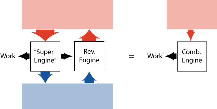
Most of the work (in a broad sense) that facilitates the spontaneous processes on our little planet (like life and the weather) can be traced back to one single source: the Sun-Earth heat engine. "Hot" energy (in the form of light) of about 6000 degrees Kelvin continuously strikes the Earth from the direction of the sun. At about the same pace "cold" energy (of about 250 degrees Kelvin) is radiated from the Earth back into outer space. Somewhere in between we and nature tap into this flow of energy to make things happen (or to store it for later use).
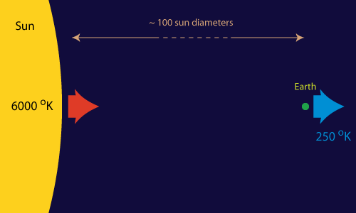
From the considerations in the previous section, the maximum efficiency of the Sun-Earth engine can easily be calculated to be
(49)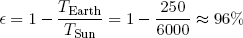 .
.
But wait a second, what do we mean by "hot" when we talk about radiation from the Sun?
Well, the energy of a "lump of light" (called a photon) is proportional to its frequency. The light quanta that are emitted from the Sun have frequencies mainly in the visible spectrum (i.e. red to blue) and in the ultraviolet. Light radiated from the Earth on the other hand mainly contains low frequency infrared photons (i.e what the police and the army uses to see people in the dark).
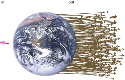
Now, the amount of energy that strikes the Earth is about the same as the amount that leaves it (otherwise it would get very hot out there). But since the incoming light has a higher energy (or frequency) per particle than the outgoing light. We must have that a big number of particles is going out for every particle that comes in (see figure 11). The entropy of light radiation is directly proportional to the number of photons it contains, so low entropy comes in, high entropy goes out. This is what drives the world (not energy, as opposed to popular believe). Don't try to safe energy, try to safe low entropy!
Before we wrap up, I quickly want to mention that there is yet another big heat engine operational on our planet - or should I say in our planet. Things like the slow drift of continents (plate tectonics), volcanic eruptions, and the formation of mountains, are driven by a "heat engine" that runs between the hot, partly molten core of our planet and the cold solidified surface we live on.
The rest of the universe
"So," you say, "you are telling me that we live in a world that is completely driven by the tendency to move from low entropy to high entropy, but tell me, where does all this hot, low entropy, energy come from in the first place?"
The truth is, we really don't know. A fact of history is that the universe started out in a very dense, hot and thus low entropy state. Then, for unknown reason, the space that contains all this hot matter/energy started to expand very quickly (and is still doing this). Like an expanding gas (or a relaxing rubber band for that matter), the energy in the universe started to cool down. However the expansion was so fast (i.e. not adiabatic) that the tendency to equilibrate could not keep up with the rate of expansion (a bit like when you land on your belly in a swimming pool and the water has no time to flow around you, ouch; maybe that's why they call it the "big bang"). The density fluctuations that emerged, were unstable and collapsed under the weak but ever present influence of gravitational attraction. From these density fluctuations the first stars emerged. Planets like ours were formed a few generations of stars later (from stardust of stars that exploded in the final stage of their existence).
And there we are, still not in equilibrium, driven by the tendency to get there. No one knows where the story will end, or even if it will end.
For a more detailed account of the early universe, its development, the state of affairs at present and the importance of the second law to life, I can recommend a recent review article published by Charles H. Lineweaver and Chas. A. Egan in the Physics of Life journal.
References
- Richard P. Feynman, Robert B. Leighton and Matthew Sands, The Feynman Lectures on Physics, Vol. I, Addison-Wesley (2006)
- Daniel V. Schroeder, Thermal Physics, Addison Wesley Longman (2000)
- L. D. Landau and E. M. Lifshitz, Statistical Physics (3rd edition, part 1), Vol. 5 of the Landau and Lifshitz Course of Theoretical Physics
- David Chandler, Introduction to Modern Statistical Mechanics, Oxford University Press (1987)
- Charles H. Lineweaver and Chas A. Egan, Life, gravity and the second law of thermodynamics, Physics of Life Reviews 5 (2008), p. 225–242
