Your everyday world from a physicist's perspective
Candle flames in one-g
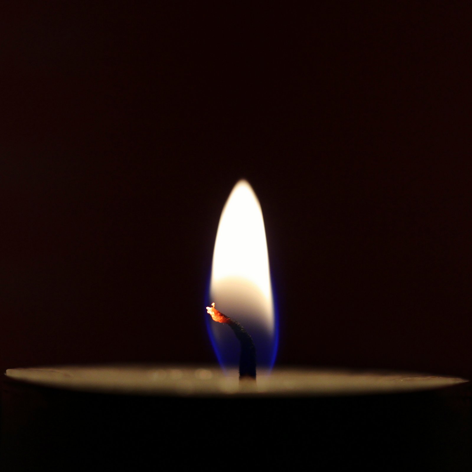
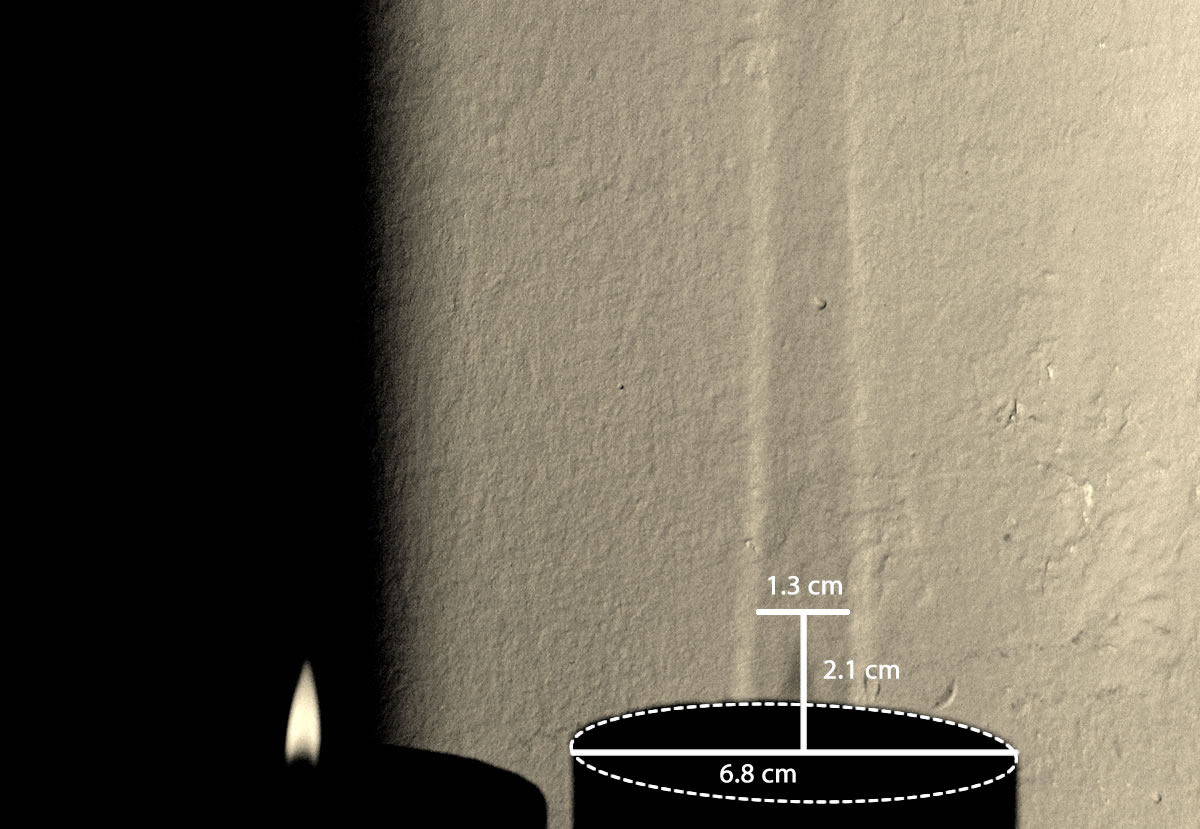
I love to stare into a candle flame and think of how it manages to preserve its own brilliance by a delicate interplay between chemistry [1, 2] and physics. People usually burn candles when it is dark, but it is only in bright sunlight that some of their best kept secrets are revealed (see figure 2).
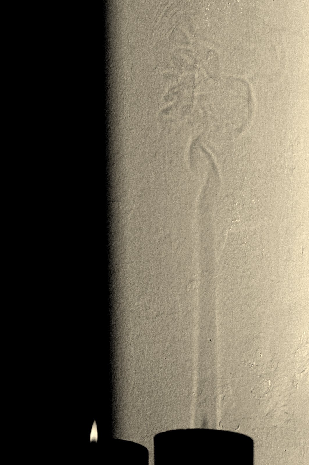
The first thing to notice about the shadow on the wall, is the long vertical column with bright edges that encapsulates the candle flame and ends in a wiggly mess at about 20 cm above the flame tip. This is a 'convection plume' of hot air that rises because of its low density compared to the surrounding cold air (like a hot air balloon). Because the index of refraction of a gas changes with temperature, the plume acts as a strangely shaped lens, with the bright lines in the image corresponding to parts in the plume where the second spatial derivative (slope of the slope) of the temperature profile is high.
The role of the rising plume in determining the structure and intensity of the flame becomes clear when we partly block it by placing some aluminum foil around the base, as shown in figure 3.
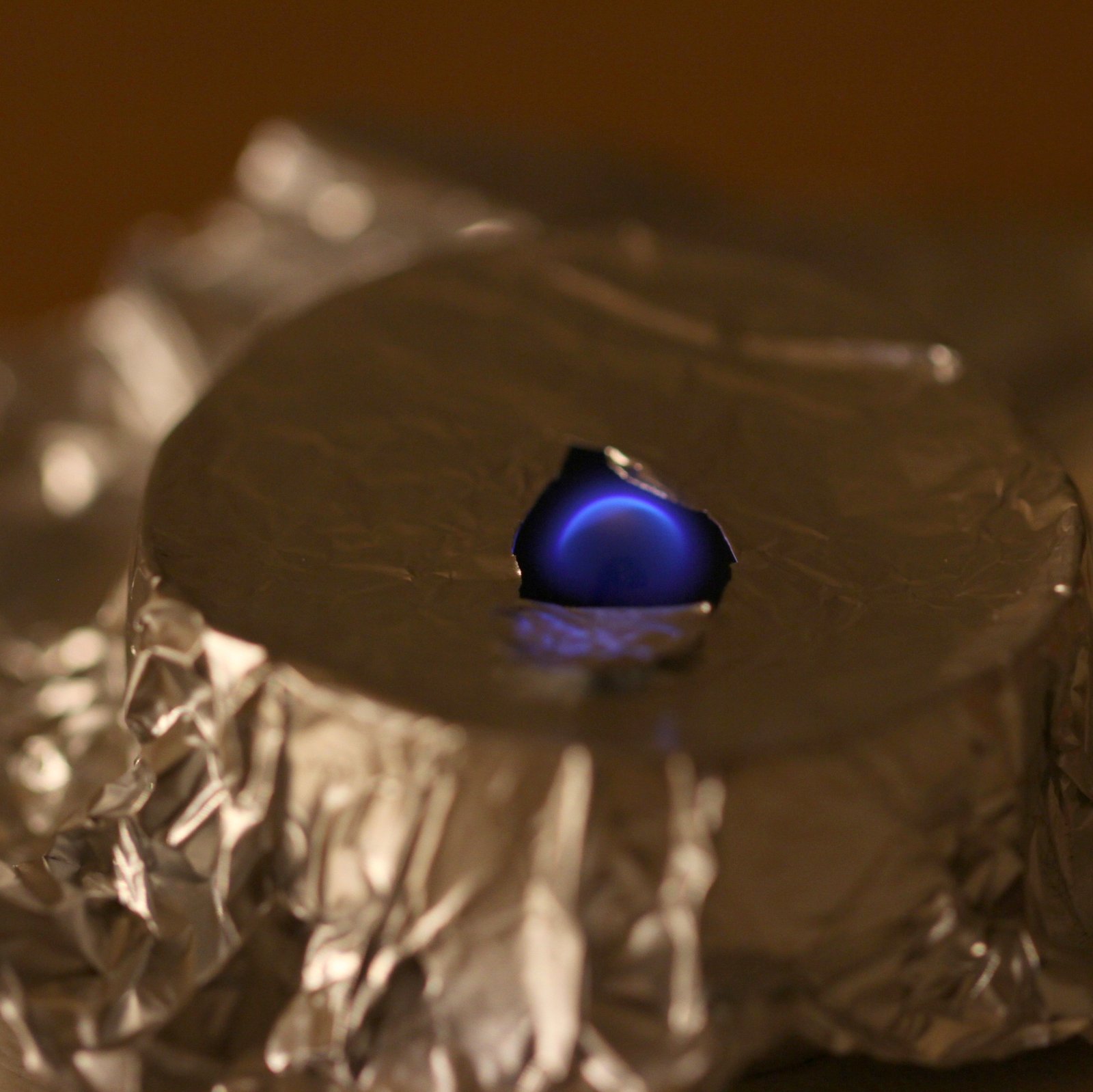
When the aluminium foil is in place (making sure that no fresh air can enter near the base) only a faint blue glow remains. This is similar to how a candle burns in free fall (zero-g) in the international space station. The typical blue color indicates a complete combustion reaction reminiscent of the one you see in a gas stove.
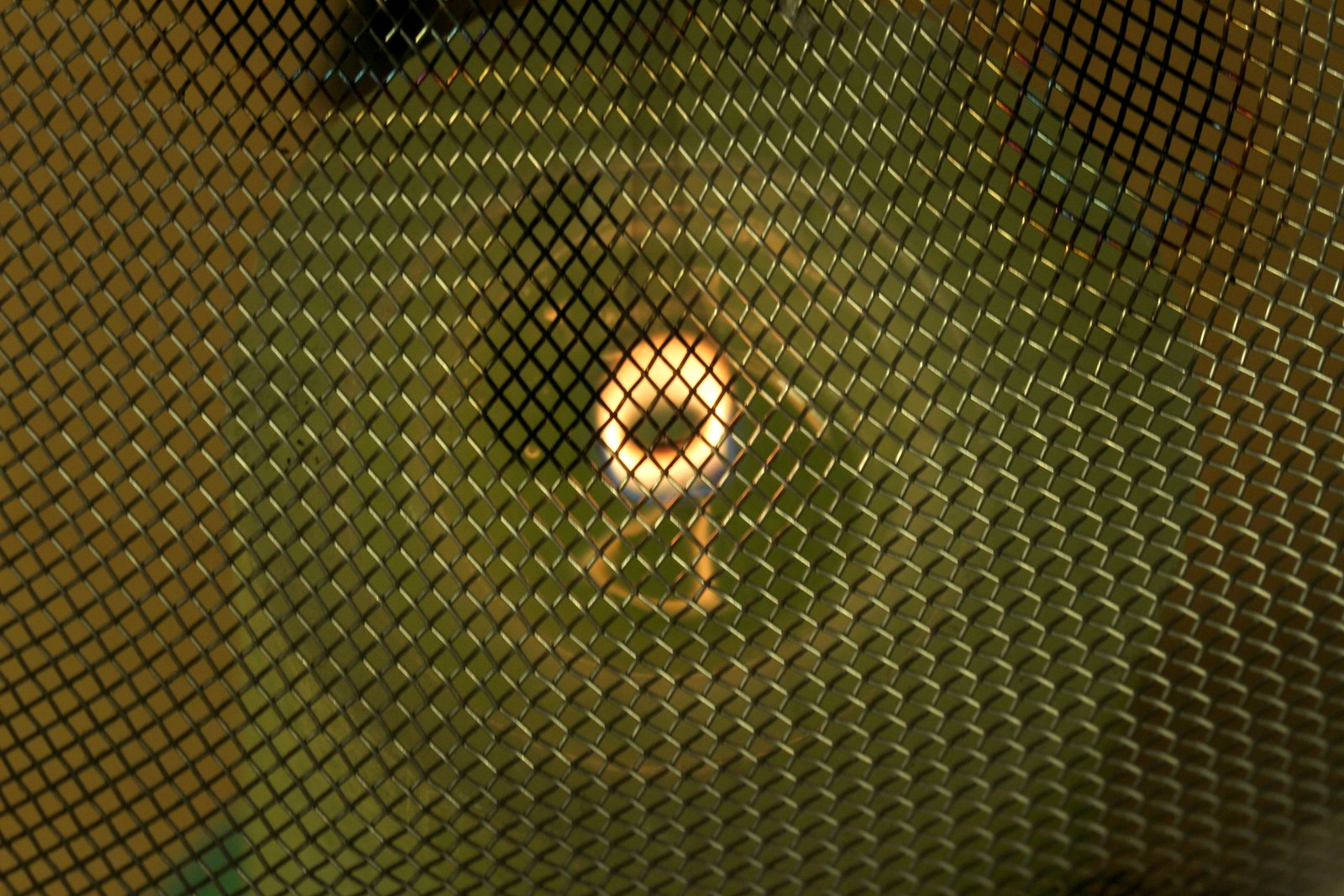
So what about the bright yellow light? A hint can be found by looking carefully at the shadow of the flame in figure 2. The bright part of the flame is dark in its shadow!
In figure 4 I used a metal sieve from my kitchen to take a look into the flame without disturbing it too much (before you try this at home, be aware of the fact that the heat from the flame will leave permanent colorized spots on your sieve, oops).
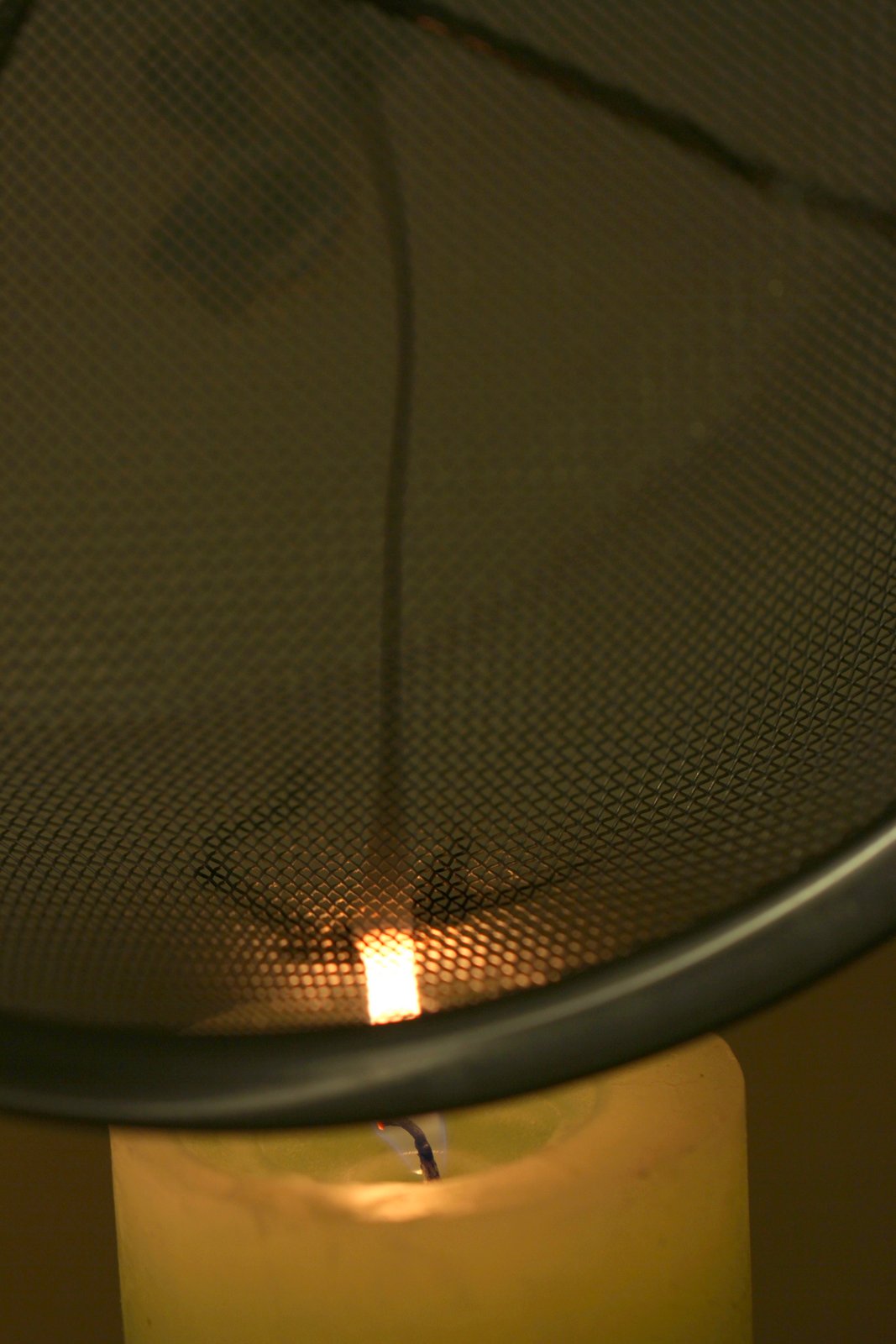
A stream of black particles emerges from the bright part of the flame. This 'soot' originates from an incomplete combustion reaction taking place within the flame (where the oxygen concentration is relatively low). When these particles are heated by the surrounding flame, they start to glow like hot coals -- giving rise to the familiar white-yellow flame color. Note that under normal circumstances, no soot escapes from the candle flame. Everything is burned at the edge of the flame, where there is sufficient supply of oxygen.
Actually, in the old days one had to periodically cut the wick of a candle to prevent emission of soot. The dimensions of the wick determine the amount of fuel available for burning [6]. When the wick is too long, the supply of oxygen cannot keep up with the supply of fuel, and some soot will get through unburned. In modern candles, the wick is designed to always curl to one side, so that its tip is continuously burned away by the hot edge of the flame: a self-trimming wick, very smart!
Now that we have a rough idea of how heat and mass flow in and around a candle flame, we can try to find a more detailed description.
I. The thermal convection plume
Because of the importance of the rising air in determining the shape of a candle flame, it makes sense to start our theoretical exposition with a model of this 'thermal plume'.
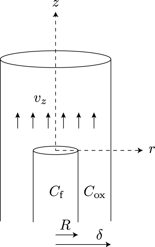
To keep the problem manageable we strip down the complex nature of a burning candle until we are left with a picture that has just enough "clothes on" to capture the physics of the plume. Figure 5 shows the picture I have in mind.
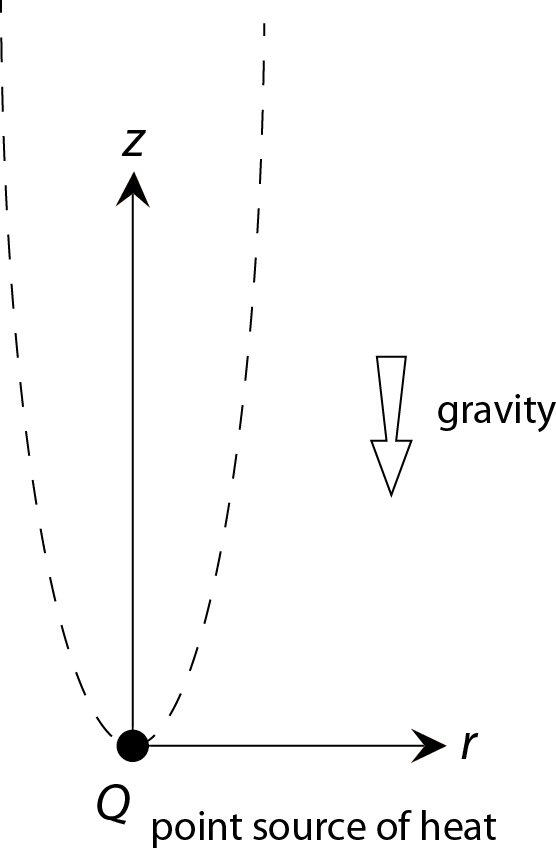
One simplification is that we will assume that all the heat produced in the flame comes from a single point in space. From here we will try to find a steady, axis symmetric flow profile that satisfies the local conservation laws -- mass, momentum and energy -- and the 'boundary conditions' imposed by the presence of the heat source and the fact that nothing happens at large r.
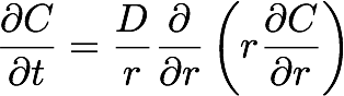
Mathematically, the conservation of fluid (in cylindrical coordinates) can be written as
(1) ,
,
where r and z are respectively the coordinate in the radial direction and the vertical direction (see figure 5) and vr(r,z) and vz(r,z) are the fluid velocities in these directions.
The conservation of momentum in the vertical direction can be written as
(2) ,
,
where ν is the kinematic viscosity of the fluid (a measure of the "diffusion" of momentum to neighboring fluid), g is the gravitational constant, β is the thermal expansion coefficient of the fluid and (T-T∞) is the relative increase in temperature. The last term in equation 2 represents the temperature dependent buoyancy force.
Similarly, we write for the conservation of (heat) energy
(3) ,
,
where α denotes the thermal diffusivity of the fluid.
Note that we assumed that the different fluid parameters in this model do not depend on the local temperature (which is only approximately true) and that gradients in the vertical direction are negligible compared to those in the radial direction (only valid some distance above the source).
We have to supplement these equations with the appropriate boundary conditions. At r = 0 we have
(4)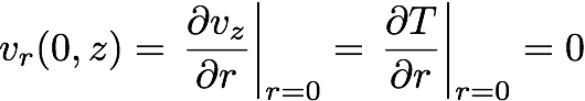 ,
,
because of the axial symmetry, while at r → ∞ we have the "nothing has changed" condition
(5) .
.
Finally, the heat flux Q(z) through a horizontal plane z above the heat source can be written as
(6)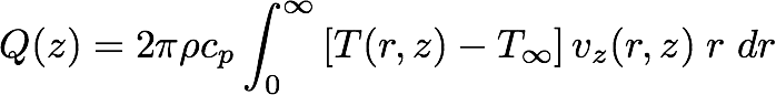 ,
,
where ρ and cp are respectively the density and the specific heat capacity of the fluid. Since the only source of heat is the point source at the origin, Q(z) must be constant and equal to the produced heat Q for all z > 0.
A scaling argument
Although it is not so hard to write down the equations we have to solve, it is certainly not straightforward to find the solution to this coupled set of partial differential equations. However, it is possible to get a first rough idea of how the solution behaves by balancing the 'order of magnitudes' of the different terms. A game physicists love to play.
We start with equation 1 for the conservation of fluid, to find our first order of magnitude balance:
(7)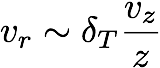 ,
,
where δT is the 'typical width' of the thermal plume at a distance z above the point source (note that we don't care about signs and pre-factors in these kind of arguments). Equation 2 gives us two possibilities, (a) the driving buoyancy force is balanced by viscous drag (the first term on the right), so that
(8a)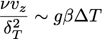 .
.
or (b) the buoyancy term is balanced by the 'inertia' terms on the left,
(8b)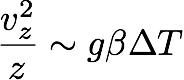 .
.
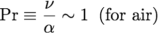
This freedom corresponds to the existence of two limiting cases. One can show that case (a) holds for liquids in which ν/α >> 1 and case (b) for liquids with ν/α << 1. This 'dimensionless' ratio is called the Prandtl number ('Pr') and it signifies the relative importance of momentum diffusion versus thermal diffusion in a fluid. Water (at room temperature) is an example of a high Pr-number fluid, while liquid metals are low Pr-number fluids. For gasses we have Pr ~ 1.
Our last differential equation, equation 3, gives
(9)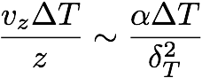 .
.
We now have three equations and four 'unknowns' (vr, δT, vz and T). To close the problem we need one more equation. It is equation 6 for the global conservation of heat flux that does the job,
(10)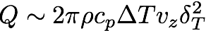 .
.
If we solve this set of equations we find, for case (a),
(11a)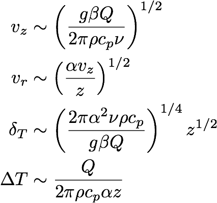 ,
,
and for case (b),
(11b)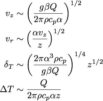 .
.
These equations tell us how the magnitudes of the different variables scale with the parameters and the height z above the heat source. Note that the two cases look very similar. The only difference is the number of α and ν factors. For a candle in air we have Pr = 0.7 (which is about 1),
(12) ,
,
so that for our purposes we can safely set ν = α, making 11a and 11b indistinguishable.
Finally note that in this model the width of the plume increases as the square root of z, while in the experiment (figure 2) the width seems to be approximately constant. This discrepancy can be qualitatively understood from the scaling relations by realizing that, for a gas, most properties actually vary strongly with temperature. We have roughly ν ~ T3/2, ρ ~ 1/T and β ~ 1/T (with T in degrees Kelvin). Since the temperature at the flame tip can be as high as 800 °C and decreases to room temperature at greater heights, this provides a non-negligible correction to the plume width δ(z) (mainly through the ν3 term). We will come back to this point near the end of this chapter, where we make a one-to-one comparison with the experiment.
Transition to turbulence
Although the equations of motion for a fluid usually allow for a steady solution, this does not mean that the actual flow will be steady. As we saw in the experiment with the tumbling book, the motion predicted by Newton's laws can be unstable with respect to small perturbations. Generally, a motion is susceptible to destabilization when the frictional damping is small compared to the momentum of the body. For our thermal plume we can estimate this ratio (inertia/damping) as
(13)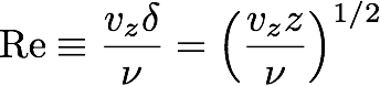 .
.
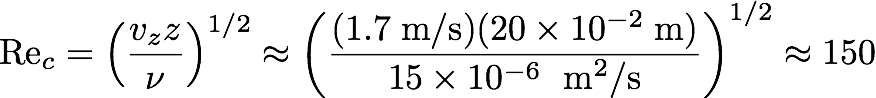
This dimensionless number is named after Osborne Reynolds (1842 - 1912), who used the concept to describe the universal behavior of the transition from 'laminar flow' to 'turbulent flow' in fluids driven through pipes. In many flow experiments one finds that the transition to turbulence occurs around Rec ~ 100. Since our local Reynolds number increases with z, we can expect the flow profile to become unstable at some point.
In the shadowgraph of figure 2 we see that the plume starts to wiggle at about 20 cm above the flame base. If we assume that at this height, the plume has cooled down to about room temperature, we find (using the properties of air at 20°C and taking Q ~ 10 W)
(14)
Self similar solution
We can now go one step beyond the scaling arguments and actually solve the set of equations (1, 2 and 3). To do this, we will assume that the shape of the plume is the same at all heights, provided that we rescale the r- and z-axis in such a way as to satisfy the scaling relations stated in equation 11. In particular, this means that the r-axis should be rescaled with the plume width δ. To this end we define
(15)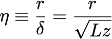 ,
,
where the constant
(16)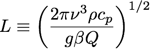
has the units of a length (L ~ 10-300 μm in our case) and sets the distance from the source where our assumption that vertical gradients (~1/z) are negligible compared to radial gradients (~1/δ), starts to be valid.
We will start with equation 1 for the conservation of fluid. This equation can be satisfied by assuming that the vertical and radial velocity can be written as derivatives of some (to be determined) function Ψ(r,z). We take
(17)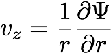
and
(18)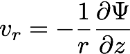 .
.
Now, to make sure that vz(0) does not change with height (as indicated by the scaling for vz), this 'stream function' must be of the form
(19)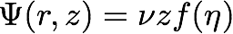 ,
,
where f(η) is some function of the rescaled radial position η that contains the shape of the plume. Plugging equation 19 into equations 17 and 18 we find
(20)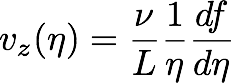
and
(21)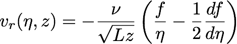 ,
,
which both satisfy the scaling laws formulated in equation 11.
Similarly, the temperature difference (T - T∞) can be formally written as
(22)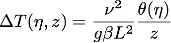 .
.
If we now substitute equations 20 - 22 into equations 2 and 3 and work out all the derivatives, we end up with two "ordinary" differential equations for the 'shape functions' f(η) and Θ(η):
(23)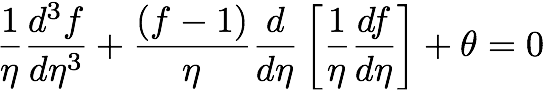
and
(24)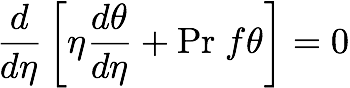 ,
,
where Pr denotes Prandtl's ratio ν/α. The boundary conditions can also be rewritten in terms of f and Θ,
(25)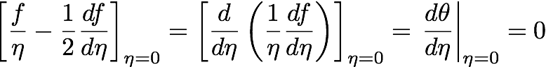 ;
;
(26)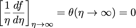 ;
;
(27) .
.
We managed to reduce the number of variables from two (r and z) to one (η), but the resulting equations are certainly not trivial to solve generally. In a paper from 1963, Fujii solved these equations for the special cases Pr = 1 and Pr = 2 [3]. To give a flavor, for Pr = 1 he found
(28)
and
(29) .
.
For other Pr-numbers we can resort to a numerical 'shooting' method, in which one repeatedly "guesses" values for f'/η (i.e. vz) and θ at η = 0, until one finds a solution that satisfies both the conditions at infinity (equation 26) and the integral condition (equation 27).
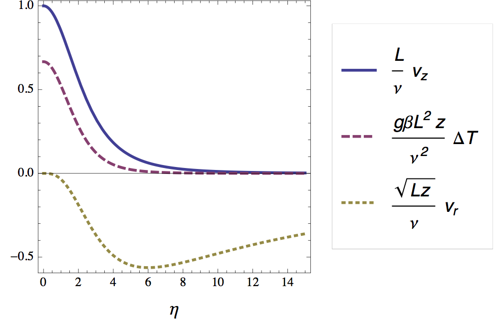
In figure 6 I plotted the velocity and temperature profile as a function of the (rescaled) radial distance.
Optical signature of the plume
As mentioned briefly in the introduction, the bright lines in the shadow in figure 2 correspond to positions in the radial temperature profile where its second derivative is high. For air (Pr = 0.7) we find -- using the numerical shooting method -- that this maximum lies at η ≈ 2.8. According to the definition of η this means that the horizontal distance W (= 2ηδ) between the bright lines should be approximately
(30)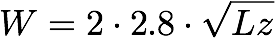 .
.
In the section on scaling we noted that L actually varies strongly with temperature (and therefore with z). We can now try to quantify this dependence.
First we need to know how the temperature varies with height. T also depends on r, but we will assume that the properties inside the plume are dominated by the central temperature Tmax. According to our scaling relation, Tmax then has to satisfy
(31)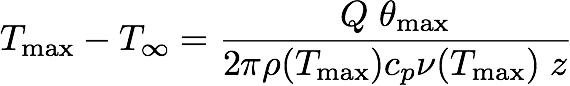 .
.
where θmax is the maximum in the shape function (which is 0.48 for Pr = 0.7). In table 1 I summarized some experimental data (from the Engineering Toolbox website) on how the parameters in equation 31 vary with temperature (approximately).
| Specific gas constant Rs | 287 [J kg−1 K−1] |
| Atmospheric pressure Pa | 101 325 [Pa] |
| Density ρ | Pa / (RsT) [kg/m3] |
| Specific heat constant cp | 1.0 [kJ kg-1 K-1] |
| Kinematic viscosity ν (300K - 1400K) | -8.86 x 10⁻⁶ + 6.10 x 10⁻⁸ T + 6.59 x 10⁻¹¹ T2 [m2/s] |
| Thermal expansion coefficient β | 1/T [K-1] |
Using this data we can numerically solve equation 31 for Tmax. Figure 7 shows the result (where I chose to measure z from the flame base and estimated Q to be about 10 W [5]).
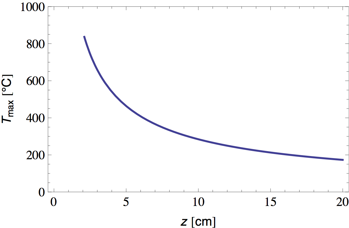
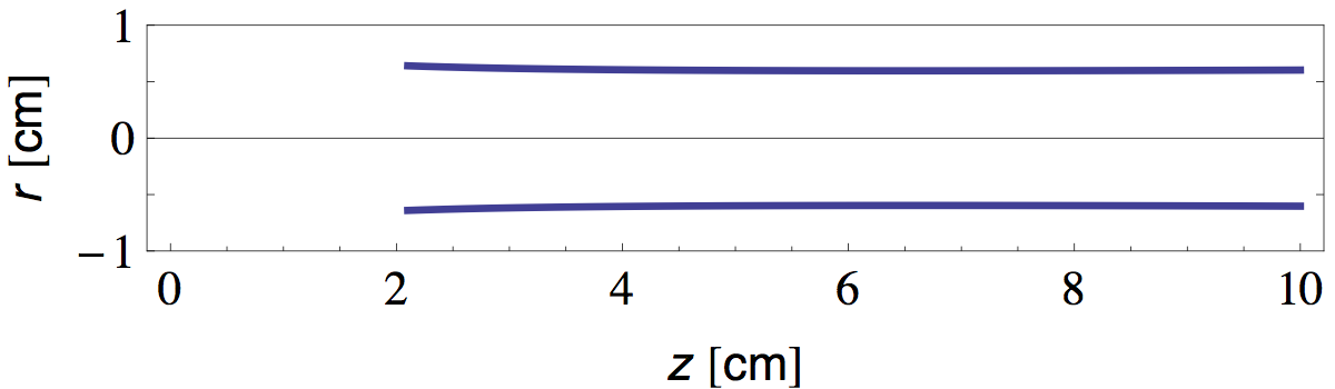
We see that the temperature at the flame tip is about 800 °C and diminishes as ~1/z at greater distances. Now that we have T(z), it is straightforward to calculate L(z) and W(z) from equations 16 and 30 and the properties of air tabulated in table 1. In figure 8 I plotted the radial position of the bright "plume lines" predicted in this manner.
Note that in discussion above, we implicitly assumed that all parameters vary "sufficiently" slow with height and radial distance, so that the plume profile is still (at least approximately) given by the self similar solution with constant parameters derived in the previous section.
Experiment will be our judge.
Comparing figures 8 and 9, we see that theory and experiment match surprisingly well, considering the crude approximations we made along the way.
Now that we have some confidence in our plume model, we can try to extract flow parameters that are not directly accessible in our experiments. Crucial in the next section will be the typical air velocity vz inside the plume. Using the properties of air at 800°C (ν ~ 1.4x10⁻⁴ m2/s and L ~ 250 μm) we find a rise velocity of about vz = 0.5 m/s near the flame tip.
II. Shape of the candle flame
A candle flame is an example of a 'diffusion flame'. This means that the rate at which fuel is burned is determined by the radial diffusion of wax vapor (the fuel) outward and oxygen inward. A mixture of fuel and oxygen burns most intense when the ratio of oxygen supply to fuel supply is such that they can completely react to H2O and CO2, i.e. with no "leftovers". This so called 'stoichiometric mixture' condition determines the position of the hot flame edge of a diffusion flame. On the inside of this edge there is only enough oxygen for an incomplete combustion reaction, which produces the yellow glowing soot we all love.
In this section I would like to show how the combination of upward convection and radial diffusion gives rise to the typical shape of a candle flame. To this end I will employ an elementary model that was introduced by Burke and Schumann in 1928 [4]. Figure 11 shows a schematic outline of the model.
Burke and Schumann imagined two coaxial tubes with radii R and δ. The inner tube holds fuel-rich gas, while the outer tube holds oxygen-rich gas. Both gasses are convected upward with a constant velocity vz. The inner tube stops at z = 0, allowing the gasses to interdiffuse freely from this point onward. The flame front is defined as the collection of points where the diffusion of fuel and oxygen results in a stoichiometric mixture.
Mathematically, 'cylindrical' diffusion of a gas can be described by a differential equation of the form
(32) ,
,
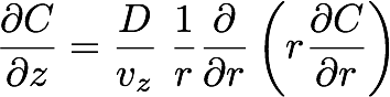
which states that the time rate of change of the concentration C(r,t) at any point in space is given by the difference in concentration gradient between the left side and right side of this point, multiplied by a diffusion "constant" D that depends on the physical surroundings of the gas.
To take into account the constant upward convection, we can simply substitute t by z/vz in equation 32 (as if we were moving with the flow),
(33) .
.
The next step would be to solve an equation of this type for both Cf and Cox (with the appropriate initial and boundary conditions) and then to trace out the flame front defined by the reaction stoichiometry of paraffin wax (see [2] for a more detailed account of the chemistry of candles),
(34) .
.
Following Burke and Schumann we can take a neat shortcut in this diffusion problem. Instead of solving two separate equations for Cf and Cox, we can exploit the linearity of equation 33, and solve a single equation for C ≡ Cf - Cox/s. Where s (≈ 3) denotes the mass ratio of oxygen to wax in the combustion reaction. From this perspective, the flame edge will be given by the condition C(r,z) = 0. Note that we must assume here that both gasses have approximately the same diffusion constant.
With initial condition [ C(r, 0) = Cf(0) for 0 < r < R, C(r, 0) = -Cox(0)/s for R < r < δ ] and boundary conditions
(35)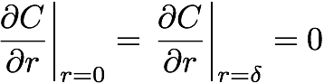 ,
,
the solution to equation 33 can be written as
(36)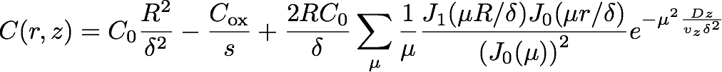 ,
,
where C0 ≡ Cf(0) + Cox(0)/s. Jn(x) are the so called 'Bessel functions of the first kind', which often appear in problems with radial symmetry. The sum in the last term runs over the infinite number of zeros μ of the Bessel function J1(x). A graphical representation of this solution at different heights is shown in figure 12. The small wiggles on the initial step function are due to the fact that I let my computer evaluate only the first 100 terms in the infinite sum. These artificial wiggles are quickly smoothened out at greater heights.
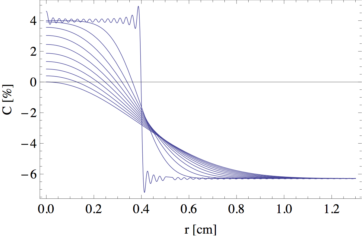
The intersections of the blue curves with the black line C(r) = 0 are the points that define the edge of the flame. In figure 13 I tracked this intersection point as a function of z to find the full outline.
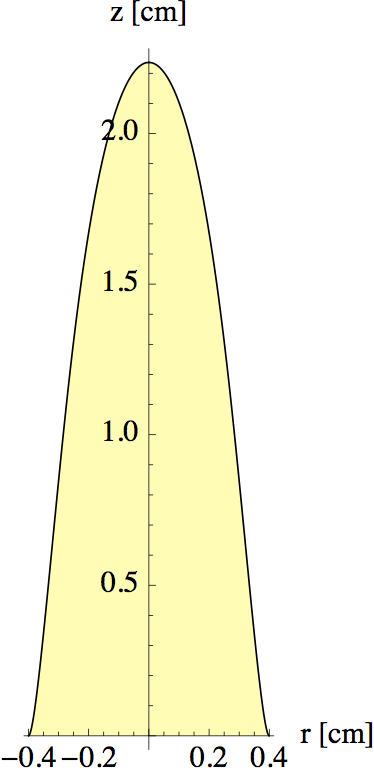
In making figures 12 and 13, I played a bit with the initial concentration of fuel to get a realistic value for the flame height (with vz = 0.5 m/s, as found in the previous section). The diffusion constant was estimated to be D = 1x10⁻⁴ at 800°C (for a gas D ~ ν, so we can use table 1). Note that our model only captures the flame shape above the wick, where there is no new fuel produced. In the region surrounding the wick things are more complicated.
If δ is sufficiently large (so that the outer edge is not "felt"), it turns out that the height H of the flame is given by the simple formula
(37)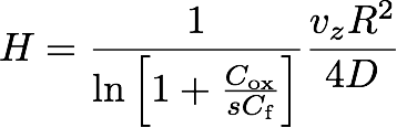 ,
,
which can be understood as a "competition" between the vertical convection time scale tconv = H/vz and the radial diffusion time scale tdiff = R2/4D. Together with the existence of a buoyancy driven convection plume, the competition between these time scales captures the essence of the special appearance of candle flames in one-g.
Bonus movie: relighting a candle from a distance
References
- Michael Faraday, The Chemical History of a Candle (read online), London, Chatto & Windus (1908)
- Klaus Roth, Chemistry of the Christmas Candle (part 1, part 2, part 3), translated by W.E. Russey, Chemie in unserer Zeit/Wiley-VCH (2011)
- T. Fujii, Theory of the steady laminar natural convection above a horizontal line heat source and a point heat source (doi), Int. J. Heat Mass Transfer 6, 597 (1963)
- S. P. Burke and T. E. W. Schumann, Diffusion Flames (doi), Industrial and engineering chemistry 20, 998 (1928)
- A. Hamins, M. Bundy and S. E. Dillon, Characterization of Candle Flames (doi), Journal of Fire Protection Engineering 15, 265 (2005)
- P. B. Sunderland, J.G. Quintiere, G. A. Tabaka, D. Lian and C. W. Chiu, Analysis and measurement of candle flame shapes (doi), Proc. Combustion Institute 33, 2489 (2011)
